A heuristic algorithm using tree decompositions for the maximum happy vertices problem
Many problems are hard, very hard. This is not only for humans, but also for computers. Researchers have put significant effort into developing efficient algorithms for solving these hard problems. One such approach exploits a so-called tree decomposition to efficiently find solutions. However, this only works if the treewidth of the tree decomposition is sufficiently small. This requirement cannot be guaranteed in practice. In this work, we created a heuristic algorithm using tree decompositions for the maximum happy vertices problem. Our algorithm finds good solutions (but not necessarily optimal) in only a fraction of the time, even if the treewidth is unbounded.
On this page, I will explain what a tree decomposition is, how they are used to efficiently solve hard problems, and how we extended this approach to a heuristic algorithm. But first, how can we make a vertex happy?
The Maximum Happy Vertices Problem
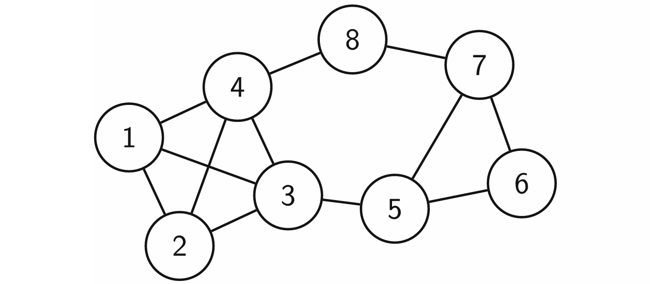
Before we can talk about happy vertices, we need to talk about graphs. A graph is a mathematical structure that is used to describe interconnected objects, for example people and their friends. Formally, a graph exists of vertices which represent the objects (e.g., people) and edges which connect the vertices (e.g., which persons are friends). These graphs are typically drawn as some connected circles, in which the circles are the vertices and their connections are the edges. Below figure shows an example of such graph.
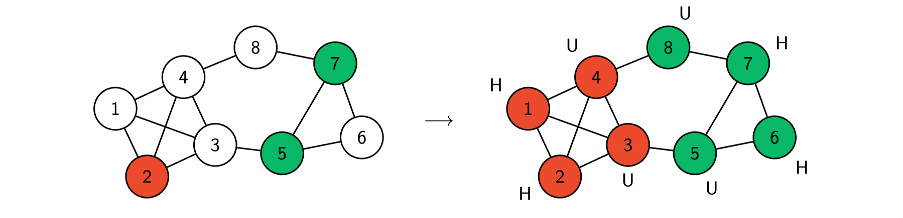
The maximum happy vertices problem considers graphs in which the vertices are coloured, and we say that a vertex is happy if it has the same colour as all its neighbours (i.e., the vertices it is connected to). For example, imagine you need to assign the seat arrangement on your wedding. The vertices could represent the invitees, the edges who are friends to each other, and the colour represents the table to which you assign the invitee. An invitee/vertex is happy if he sits together with many friends. Given a graph in which a small set of the vertices are coloured, the maximum happy vertices problem requires you to colour all the remaining vertices such that the number of happy vertices is maximised, such that the maximum number of invitees at your wedding is happy with their seat. An example is given below.
The Tree Decompositions
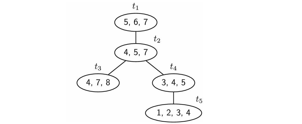
Before you can understand tree decompositions, you must know what a tree is. A tree is graph that does not contain any cycles. The graph in Fig. 1 is not a tree because it contains multiple cycles, one of which is the path from 5 to 6 to 7 and back to 5. The tree decomposition of a graph is a tree, in which each vertex represents a subset of the vertices of the graph, also called a bag. We call the vertices of this tree nodes to distinguish them from the vertices of the graph. An example of a tree decomposition is given in Fig. 3, in which the numbers inside the nodes represent the subset of vertices related to that node. For example, the bag of node \(t_3\) has vertices 4, 7 and 8. An important property of tree decompositions is the width, which equals the size of the largest bag minus 1. The tree decomposition below has a width of 3, because the largest bag in \(t_5\) contains 4 vertices.
However, not every tree with bags is a tree decomposition, it must satisfy three properties:
- Every vertex in the graph must be part of at least one bag.
- Every pair of vertices in the graph that are connected must be at least once in the same bag. For example, vertices 3 and 4 are connected, and are both part of node \(t_4\).
- For each vertex in the graph, then the nodes which contain that vertex must be connected. For example, vertex 4 is in nodes \(t_2\), \(t_3\), \(t_4\) and \(t_5\), which are all connected. If vertex for was not in node \(t_4\), we would not have a valid tree decomposition.
Tree Decompositions to Efficiently Solve Hard Problems
Tree decompositions are relatively complex structures. However, their properties allow for a key feature: each bag separates the graph in two parts. For example, the vertices in node \(t_4\) in Fig. 3 separate the graph into the sets {1, 2} and {6, 7, 8}. All paths between two vertices of each set must pass one of the vertices in node \(t_4\)! For the maximum happy vertices problem, this feature means that if the colours of vertices 3, 4 and 5 are known, the best possible colouring of vertices {1, 2} has no influence on the best colouring of vertices {6, 7, 8}.
Algorithms exploit this information bottleneck to efficiently colour the vertices. Starting from the bottom nodes of the tree (also called leaves), the algorithm will create all possible colourings of the vertices in that node. Moving up the tree, the algorithm will continuously create all possible colourings for the vertices in the bag, and combine them with all the colourings of the previous node such that the number of happy vertices is maximised. For example, we need to process node \(t_4\) and have 2 colours. We consider all 8 possible colourings of the vertices 3, 4 and 5 in node \(t_4\). Then, we combine each colouring with the colours for vertices 1 and 2 which we already find in leave node \(t_5\) such that the number of happy vertices is maximised. By continuing this process until we reach the top of the tree (the root), we will find the best colouring for all the vertices in the original graph.
This probably sounds like a very convoluted way to colour the vertices. So why is this algorithm so good? Generally speaking, an algorithm will take more time the more vertices the graph has. For the maximum happy vertices problem, any exact algorithm requires exponentially more time as the number of vertices increases (except if P=NP). However, for the algorithm using the tree decomposition, the required time increases only linearly as the number of vertices increases, which is much faster than exponential!
Our Heuristic algorithm
However, there is a catch: the algorithm still has an exponential runtime, not relative to the number of vertices but relative to the width of the tree decomposition. This is because in every node we need to consider all possible colour assignments to the vertices. In the example above, we considered node \(t_4\) with vertices 3, 4 and 5 and two colours. Thus, there are two options for vertex 3, two for vertex 4 and two for vertex 5. In total, this is \(2\cdot 2 \cdot 2 = 2^3\) possibilities. In general, if there are \(k\) colours and the width of the tree decomposition equals \(w\), then in any given node we must consider at most \(k^{w+1}\) possible colourings. There is our exponential!
Our goal was to remove this exponential dependency and make the algorithm more efficient, at the cost of no longer being able to find the optimal solutions. We did so by only looking at the most promising colourings of each node. Specifically, the algorithm requires a value \(W\) which defines the number of colourings to look at. For example, if \(W=4\), then we would look at 4 out of the 8 possible colourings in node \(t_4\).
Most importantly, \(W\) is an upper limit on the number of colourings to consider in each node. If \(W\) is large enough, all possibilities will be considered, and our algorithm guarantees to find the optimal solution. This is the case if
\[W \geq (2k)^{w+1}\]
with \(k\) the number of colours and \(w\) the width of the tee decomposition. Thus, our algorithm can be used to find either a heuristic or approximate solution by only changing the value of \(W\)!