Towards Contextual, Cost-Efficient Predictive Maintenance in Heavy-Duty Trucks
Complex, industrial machines are everywhere nowadays: electrical motors, compressors, robotic arms, injection moulding machines, 3D printers, etc. Here, we will focus on SCANIA trucks driving under heavy conditions. One must be able to predict the health status of the machine in order to plan maintenance before the machine breaks, thereby reducing the downtime as well as the costs. Engineers have added many sensors within the trucks measuring all kinds of properties of the truck such as temperatures and pressures. This data then enables to develop automated solutions to predict failures.
This work was part of the IDA 2024 industrial challenge. Below I will first discuss the problem, and then present our solution.
Problem formulation
There are two types of observations data given: (1) operational readouts and (2) truck specification.
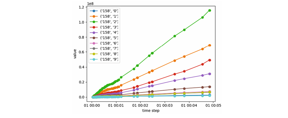
The operational readouts measure several parameters while the truck is driving. To limit storage requirements, experts defined a number of intervals in which the parameters can fall. For example, a temperature could be smaller than 20°C, between 20°C and 25°C, between 25°C and 30°C, or larger than 30°C. For each interval, a counter counts how often a measurement is taken in each interval. The operational readouts are then snapshots of these counters at irregular time intervals. In total there are 14 anonymized parameters with a variable number of intervals. An example of these readouts for a single truck is given below.
The truck specification is a static feature for each truck that does not change over time. This includes information such as the engine type, weight capacities and wheel configurations. There are 8 categorical features with variable number of categories.
The last observation of each truck is assigned one of five labels: 0 if the truck will not fail within the next 48 time steps, 1 if it will fail within the next 48 to 24 time steps, 2 if it will fail in the next 24 to 12 time steps, 3 if it will fail in the next 12 to 6 time steps, and 4 if it will fail within the next 6 time steps. Thus, classes 1, 2, 3, 4 indicate a failure with increasing severity. The goal is to predict the correct label for each truck, thus predicting if the truck will fail. A cost is defined for each of the 25 pairs of actual observations and predicted observations, in which the cost of a false negative (when the truck will fail, but you predict it won’t) is much higher than a false positive. The cost of each vehicle is summed to obtain a final score over a fleet of observations.
Transforming the operational readouts
To apply predictive models on the operational readouts, we must first transform the operational readouts. For this, we applied the following steps:
- Fill in the missing values using linear interpolation.
- Applied differencing (subtracting each value from the next one) to focus on the increase/decrease within each interval instead of the absolute counts.
- Extract segments with a fixed number of consecutive observations from the time series data.
- Compute features from each segment using tsfresh.
- Select the most important features using Kendall’s \(\tau_B\) and the Pearson correlation coefficient.
Predicting failures
Because the problem formulation is open-ended, there are multiple approaches to predict failures. Therefore, we evaluate multiple approaches and compare them to analyze the differences.
Classification models
These models directly predict the class label (0, 1, 2, 3, or 4). We use K-NN, decision trees, random forests, logistic regression, support vector machines, and XGBoosting.
Regression models
The class labels represent a severity, which is ignored by classification models. Instead, we treat these class labels as numerical values and train a regression model to predict it, and round the continuous prediction to obtain one of the class labels. As for the classification models, we use K-NN, decision trees, random forest, linear regression, support vector machines and XGBoosting.
Survival analysis
Survival analysis aims at predicting the time until failure directly (e.g., a failure will happen in 20 time steps). Then, these predictions can be transformed into class labels as described above. We use XGBoosting with the accelerated failure time model for this.
Baselines
To quantify whether the models generalize properly to unseen data, we also include a number of baselines. “Always predict X” will constantly predict label X, independent of the data. Then, we also include “Random” which selects a label uniformly at random. Similarly, “Weighted random” also samples a random class label, but weighted by the number of time each label occurs in the test data. For both random baselines, we average the total cost of 100 predictions to reduce the variance.
Dealing with the truck specification
The vehicle specification of a truck may have a huge influence on the failure potential. To take this into account, we cluster the trucks and train a model within each cluster, along with a global model for trucks that do not fit in any context. To compute the distance between two trucks, we count how many of the vehicle specifications have the same value, and combine it with the differences in trend of the readout data. Once we have the distance between each pair of trucks, we can apply hierarchical clustering to iteratively combine trucks to form clusters. Finally, we train one of the models described above to predict failures within each cluster independently.
The results
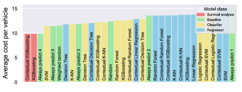
The results of this experiment are shown in Fig. 2 below. We can draw multiple conclusions from this figure:
- Baseline “Always predict 4” gives comparatively low average cost because of the imbalanced cost for false positives vs. false negatives.
- Survival analysis is the best model besides this baseline, although it does converge to always predict class label 4.
- Classification models generally outperform regression models, even though they do not take class severity into account.
- In general, including the vehicle specification does not have a huge impact. In general, simpler models like linear regression benefit more from context, because the data within each context is simpler than the full dataset.